이전까진 regular grid로 표현가능한 data를 처리하는 것에 특화된 convolutional network에 대해 알아봤습니다.
이런 경우는 특히 inpur variable이 굉장히 커서 fully connected network를 사용하는 것이 어려운 image를 처리하는데에 적합했습니다. convolutional network의 각 layer는 공유하는 parameter를 사용해 image의 각 position에서 local image patch가 비슷하게 진행됩니다.
이번 chapter에선 'Transformer'에 대해 알아봅니다.
transformer는 natural language processing (NLP) problems에 target되어 있고 NLP의 경우에 network input은 'words' 혹은 'word fragment'를 표현하는 고차원의 embedding의 연속입니다.
물론 language dataset은 image data의 몇몇 특징과 공통되긴 합니다. 예를 들어, input variable이 매우 크고, 모든 position에서 statistic은 비슷합니다. 예를 들어, text의 본문에 있는 모든 가능한 position에서 'dog'라는 단어의 의미를 다시 학습하는 것은 비효율적입니다. (?)
그러나 language dataset은 text sequence가 매번 다르고, image와 달리 'resize'하는 것이 쉽지 않습니다.
Processing text data
다음과 같은 passage가 있다고 가정해봅시다.
" The restaurant refused to serve me a ham sandwich because it only cooks vegetarian food. In the end, they just gave me two slices of bread. Their ambiance was just as good as the food and service."
우리는 network에게 바라는 것은 이 text가 downstream task에 적합한 representation으로 만드는 것입니다.
downstream task 중엔 해당 리뷰가 positive인지 negative인지 분류하거나, "Does the restaurant serve steak"라는 질문에 대답을 할 수 있는지 등이 있습니다.
이 때 우리는 3가지를 알 수 있습니다.
1. encoded input은 매우 매우 클 수 있다.
이 경우엔, 각 37개의 단어들은 길이가 1024인 embedding vector에 의해 표현될 수 있고, 그렇다면 그렇게 길지 않은 구절임에도 불구하고 encoded input의 길이는 37x1024=37888이 됩니다. 현실적으로 text의 크기는 훨씬 클 것이고, fully connected neural network는 실용적이지 않습니다.
2. NLP의 특징 중 하나는 각 input이 제각각 다른 길이를 가집니다.
그렇기 때문에 더욱 더 fully connected network를 사용하지 어려워집니다. 이러한 점은 다른 input position에서 단어들 사이에서 parameter를 공유해야 하게 만듭니다.
3. 언어는 그 자체로 ambiguous(모호)합니다.
pronoun 'it' 그 자체로는 syntax에 있으면 이는 무엇을 의미하는지 명확하지 않습니다. text를 이해하기 위해선, 단어 'it'은 'restaurant'단어와 어쨌든 연결되어 있어야 합니다.
transformer의 관점에서 보면, 방금 살펴본 'it'이란 단어는 나중의 단어들에 'pay attention' 해야 합니다.
이는 단어들 사이에 connection이 있어야 하고 이 connection의 힘은 그 단어들 자체에 의존하게 됩니다. 게다가, 이런 connection은 더 큰 text span으로 확장할 필요가 있습니다.
Dot-product self-attention
정리하자면 text를 다루는 model은
1. 다른 길이를 갖는 input passage를 다루기 위해 공유하는 parameter를 사용하고
2. 단어들에 따른 word representation 사이의 connection을 포함해야 합니다.
transformer는 'dot-product self-attention'을 사용해 위의 특징들을 얻을 수 있습니다.
standard neural network layer f[x]가 Dx1 input을 갖고 ReLU와 같은 activation function을 따르는 linear transformation을 적용한다고 하면

이 식을 따르게 됩니다. 여기서 β는 bias를 포함하고, Ω 는 weight를 의미합니다.
self-attention block sa[.]은 N개의 input x1,...,xN을 갖고, 각 input의 dimension은 Dx1입니다. 그리고 같은 크기의 N개의 output vector를 return합니다. NLP의 상황에서, 각 input은 word 혹은 word fragment를 포함합니다.
첫번째로, value의 set은 각 input에서 계산됩니다.

β(v)의 dimension은 Dx1이고 bias를 의미합니다. Ω(v)의 dimension은 DxD이고 weight를 의미합니다.
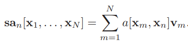
n번째 self-attention output sa(n)[x1,,,.,xN]은 모든 value v1,...,vN의 weighted sum입니다.
여기서 scalar weight a[xm,xn]은 n번째 output 이 input xm에 부여하는 attention입니다.
N weight a[.,xn]은 non-negative이며 합은 1이 됩니다.
그러므로, self-attention은 각각의 output을 만들기 위해 다른 비율로 value를 'routing'하는 것으로 볼 수 있습니다.

self-attention mechanism은 각 dimension이 D인 N개의 input (x1,...,xN) 을 갖고 N개의 value vector를 각각 갖기 위해 진행됩니다, n번째 output sa(n)[x1,...,xn]은 N value vector의 weighted sum으로 계산됩니다. 여기서 weight은 모두 양수이며 총 합은 1입니다.
a) output sa(1)[x]는 a[x1,x1]=0.1배가 첫번째 value vector에 계산되고, a[x2,x1]=0.3은 두번째 value vector에, a[x3,x1]]=0.6은 세번째 value vector에 계산됩니다.
b) output sa(2)[x]도 같은 방식으로 계산되지만 각 weight은 0.5,0.2,0.3이 됩니다.c) sa(3)[x]도 동일합니다. 각 output은 N value의 다른 routing이라고 볼 수 있습니다.
Computing and weighting values
이 식에서 볼 수 있듯 같은 weight와 bias가 각 input x(n)에 사용됩니다.
(이 때, Ω는 DxD dimension, β는 D dimension, x는 D dimension입니다)
이 계산은 lineary하게 sequence length N만큼 확장되고, 그렇기 때문에 모든 DN input을 모든 DN output에 연결하는 fully connected network보다 더 적은 parameter가 필요합니다.
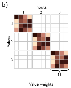
이 그림에서 볼 수 있듯 value 계산은 공유하는 parameter를 이용한 sparse matrix operation으로 볼 수 있습니다.
attention weight a[xm,xn]은 다른 input인 value와 결합됩니다.
물론 이것도 각 input의 order pair (xm,xn)에 대해 하나의 weight만 있기 때문에 input size와 상관없이 sparse합니다.
즉, attention weight의 수는 sequence length N에 quadratic하게 dependent하지만, 각 input x(n)의 length D엔 independent합니다.

a) 각 input xn은 같은 weight와 bias에 독립적으로 작동합니다. 각 output은 value의 linear combination이며 shared attention weight a[xm,xn]는 n번째 output에 대한 m번째 값의 기여도를 정의합니다.
b) 해당 matrix는 input과 value사이의 linear transformation의 sparsity를 나타냅니다.
c) 해당 matrix는 attention weights relating value와 output의 sparsity를 나타냅니다.
Computing attention weights
이전의 section에서, output은 중첩된 2개의 linear transformation으로 결과를 구합니다.
value vector β(v)+Ω(v)x(m)는 각 input xm에 대해 독립적으로 계산되고, 각 vector는 attention weight a[xm,xn]에 의해 linear하게 결합됩니다. 그러나, 전반적인 self-attention 계산은 'nonlinear'합니ㅣ다. attention weight은 그들 스스로 input의 nonlinear function입니다. 이는 hypernetwork의 예시이고, 하나의 network branch는 또다른 weight를 계산합니다.
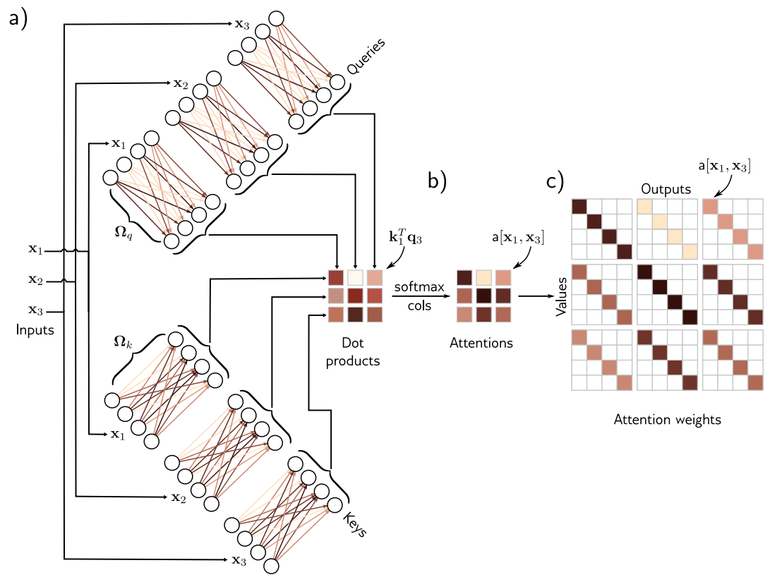
attention을 계산하기 위해, input에 2개의 linear transformation을 더 적용합니다.

{q}와 {k}는 query와 key로 쓰입니다. query와 key사이에 dot product를 계산하고 값을 softmax에 적용합니다.

dot product는 input사이의 similarity를 측정해ㅐ return하고, weight a[x,xn]은 모든 key와 n번째 query 사이의 상대적인 similarity에 따라 달라지게 됩니다.
softmax function은 key vector가 final result에 기여할 수 있도록 또다른 key vector와 경쟁하는 것으로 의미할 수 있습니다. query와 key는 그렇기 때문에 같은 dimension을 가져야 합니다. 그러나 value의 dimension은 다를 수 있지만, 보통 input과 같은 size이고, representation은 size를 바꾸지 않습니다.
Self-attention summary
n번째 output은 모든 input에 적용된 같은 linear transformation의 weighted sum입니다. 이 attention weightm은 양수이고 총 합은 1입니다. weight는 input x와 다른 input들 사이의 similarity에 따라 달라집니다. activation function은 없지만, mechanism은 dot-product와 attention weight을 구하기 위해 사용된 softmax로 인해 nonlinear이 됩니다.
이 mechanism은 우리가 언급한 조건들을 만족합니다.
1. single shared set of parameters
input N의 수에 독립적이고, 그리고 network은 다른 sequence length에도 적용할 수 있습니다.
2. input사이의 connection이 있고, connection의 strength는 attention weight을 통해 input에 따라 달라집니다.
Matrix form

위에서 다룬 computation은 각 D dimension을 가진 N input xn을 DxN matrix X로 압축한 다음 한 번에 계산할 수 있습니다.
value, query, key는 다음과 같이 계산됩니다.

이 때 1은 값이 1인 Nx1 vector입니다. 이런 경우엔 self-attention 계산은 다음과 같습니다.

이 때, function softmax는 matrix를 받아 계산하고 softmax operation을 각각 column에 맞춰 계산합니다.
이 공식에는 self-attention인 input에 기반한 3개의 product를 계산한다는 것을 강조하기 위해 input x에 대한 value, query, key의 의존성을 명시적으로 포함했습니다. 그러나 앞으론, 이 dependence를 생략하며 x를 생략하고 다음과 같이 작성합니다.

Extensions to dot-product self-attention
이전 section에서, 우린 self-attention에 대해 알아봤습니다. 실전에서 자주 쓰이는 확장된 3가지 종류에 대해 설명하겠습니다.
Positional encoding
위에서 알 수 있듯 self-attention 자체에는 input xn의 순서와 관계없이 계산이 됩니다. 그러나 input이 sentence의 word라면 이런 순서는 매우매우 중요합니다. 이런 position information을 다루기 위한 2가지 방법이 있습니다.
1. Absolute positional encodings
matrix 𝜫는 positional information을 encode하도록 input X에 더해집니다. 𝜫의 각 column은 unique해서 input sequence의 절대적인 position에 대한 정보를 포함합니다. 이 matrix는 직접 정해줄 수도 있고 train을 통해 얻을 수도 있습니다. 그리고 이 matrix는 network input에 더해지거나 모든 network layer에 더해질 수도 있습니다. 가끔은 value는 아니고 query와 key의 계산에서 X에 더해질 수도 있습니다.
2. Relative positional encodings
self-attention mechanism에서 사용되는 input은 하나의 문장일 수도, 여러 문장일 수도, 문장의 한 부분일 수도 있습니다. 그렇기 때문에 각 단어의 absolute position보다 두 input사이의 상대적인 position이 더 중요합니다. 물론 두 input의 absolute position을 알고 있으면 상관없지만, relative positional encoding은 이 정보를 직접적으로 encodin합니다. attention matrix의 각 element는 query position a와 key position b 사이의 특정 offset에 대응합니다. relative positional encoding은 각 offset에 대해 parameter πa,b를 배우고 이 값을 추가하거나, 곱하거나, 어쨌든 여러 방법으로 attention matrix를 바꿉니다.
Scaled dot-product self-attention
attention compuation에서 dot product는 큰 값을 가질 수 있고 argument를 softmax로 이동해 가장 큰 값이 완전히 지배하는 region으로 이동할 수 있습니다. softmax로 들어가는 input의 작은 변화는 이제 output에 작은 영향을 줍니다. (ex: gradient가 매우 작음). 그리고 이런 점은 model이 train하기 어렵게 만듭니다. 이를 예방하기 위해, dot product는 dimension Dq의 square root를 취한 값으로 scaling해줍니다.

다음 식은 'scaled dot-product self-attention'으로 불립니다.
Multiple heads

multiple self-attention mechanism은 보통 병렬적으로 적용되고 'multi-head self-attention'이라 불립니다. H개의 다른 value,key,query의 set이 계산됩니다.

h번째 self-attention mechansim은 다음과 같이 작용합니다.

이 때 우리는 각 head에 {β(vh), Ω(vh)}, {β(qh), Ω(qh)}, {β(kh), Ω(kh)}의 다른 parameter를 갖습니다.
보통, 만약 input xm의 dimension이 D이고 H개의 head를 갖고 있다면, value,query, key의 size는 모두 D/H가 되고, 이렇게 하면 효율적으로 구현할 수 있습니다.
이런 self-attention mechanism의 output은 수직으로 concat되고, 또다른 linear transform Ωc가 결합하게 만듭니다.

Transformer layers
self-attention은 transformer layer의 한 부분입니다. transformer는 multi-head self-attention unit으로 이루어져 있고, 그 다음엔 fully connected network mlp[.]로 들어갑니다. (각 word에 대해 별도로 작동합니다)
이 두가지 unit은 residual network입니다. 그리고 보통 self-attention과 fully connected network 이후 LayerNorm operation을 추가해줍니다. 이는 BatchNorm과 유사하지만 single input sequence에 있는 token 전체에 걸쳐 statistics을 사용합니다.
식으로 표현하자면 다음과 같습니다.

여기서 column vector xn은 full data matrix x로 부터 별도로 가져온 것입니다. 실제 network에서, data는 이런 transformer layer의 series를 통해 pass됩니다.
Transformers for natural language processing
이전 section에선 transformer layer에 대해 알아봤습니다. 이번엔 이게 NLP task에서 어떻게 사용되는지 알아보겠습니다. 전형적인 NLP pipeline은 'tokenizer'부터 시작합니다. tokenizer는 text를 word나 word fragment로 나눠줍니다. 그다음 각 token은 학습된 embedding과 mapping됩니다. 이런 embedding은 transformer layer의 series를 통해 통과됩니다.
Tokenization
이 과정에서 text를 가능한 token이 존재하는 vocabulary에 있는 더 작은 unit으로 바꿔줍니다. 우리는 이런 token이 단어를 표현한다고 가정했지만, 몇가지 어려움이 있습니다.
- 몇개의 단어들은 vocabulary에 없습니다
- punctuation을 어떻게 처리할지 분명하지 않습니다. 만약 문장이 물음표로 끝나면 우린 이 정보를 encoder 해야 합니다
- vocabulary는 같은 단어지만 다른 suffix를 가지는 여러 버전의 다양한 token이 필요합니다. 이런 관련된 variation에 대해 명확히 하는 방법이 없습니다.
실제로 vocabulary를 만드는 방법 중 하나는 'byte pair encoding'과 같은 'sub-word tokenizer' 입니다. 이 방법은 greedyㅏ게 나오는 빈번함을 토대로 공통으로 발생하는 sub-strings를 병합하는 방법입니다.
Embeddings
vocabulary v에 있는 각 token은 unique한 'word embedding'에 맵핑되고, 전체 vocabulary에 대한 embedding은 matrix Ω에 저장됩니다. 이러기 위해, N개의 input token은 처음에 matrix T에 encoding되고, 이 때 n번째 column은 n번째 token에 대응합니다. 그리고 이ㅣ는 |v|x1 one-hot vector가 됩니다. input embedding은 X= ΩT로 계산되고, Ω는 다른 network parameter와 같이 학습됩니다. 전형적인 emedding size D는 1024이고, 전형적인 total vocabulary size |v|는 30,000dlrh, main network를 하기 전에 Ω에서 학습해야 할 많은 parameter가 있습니다.
Transformer model
마지막으로, text를 표현하는 embedding matrix X는 K개의 transformer layer를 통과합니다. 이 구조가 우리가 흔히 알고 있는 'transformer model'입니다. transformer model에는 3가지 type이 있습니다.
1. 'encoder'는 text embedding을 다양한 태스크에 지원할 수 있는 representation으로 변형합니다.
2. 'decoder'는 input text에 이어지는 다음 token을 예측합니다.
3. 'encoder-decoder'는 sequence-to-sequence task에서 사용되고, 하나의 text string을 또 다른 string으로 바꿉니다. (ex)machine translation)
Encoder model example : BERT
BERT는 30,000개의 token으로 이루어져 있는 vocabulary를 사용하는 encoder model입니다. input token은 1024 dimensional word embedding으로 변형되고 24개의 transformer layer를 통과합니다. transformer layer 각각은 16개의 head를 갖는 selft-attention mechanism을 포함합니다. 각 head에 있는 query,key,value는 64 dimension을 갖습니다 (matrix Ω(vh), Ω(qh), Ω(kh)는 1024x64가 됩니다). fully connected network에 있는 single hidden layer의 dimension은 4096입니다. 총 parameter의 수는 ~340 million입니다. BERT가 소개됐을 때, 큰 모델이라 여겨졌지만, 현재 SOTA model과 비교했을 때 훨씬 작은 모델입니다.
BERT와 같은 encoder model은 'transfer learning'을 활용합니다. pre-training을 하는 동안, transformer architecture의 parameter는 text의 거대한 corpus로부터 self-supervision을 사용해 학습됩니다. 여기서 model의 goal은 language의 statistic에 대해 'general information'을 학습하는 것입니다. fine-tuning 단계에선, 결과로 나온 supervised training data의 더 작은 body를 사용해 특정 task를 풀 수 있도록 적용됩니다.

input token은 word embedding으로 변형됩니다. 여기서 word embedding은 column보단 row로 표현되고, 그렇기 대문에 "word embedding"으로 써진 box는 X^T가 됩니다. 이런 embedding은 output embedding의 set을 만들기 위해 transformer layer의 series를 통과하게 됩니다. (orange connection은 모든 token이 같은 layer에서 모든 다른 token을 attend하는 걸 의미합니다). input token의 작은 부분은 랜덤하게 <mask> token으로 바뀝니다. pre-training에서 goal은 관련된 output embedding으로 부터 사라진 word를 예측하는 것입니다. 이와 같이, output embedding은 softmax function을 통과하고, multiclass classification loss가 사용됩니다. 이 task는 missing word를 예측하기 위에 양쪽(왼쪽,오른쪽) context를 모두 사용하는 장점이 있지만, data를 효율적으로 사용하지 못하는 단점이 있습니다. 여기서 loss function에 2개의 term을 추가하려면 7개의 token을 처리해야 합니다.
Pre-training
pre-training 단계에서, network는 self-supervision을 사용해 훈련됩니다. 이ㅣ렇게 되면 manual label 없이 수많은 data를 사용할 수 있습니다. BERT에서, self-supervision task는 큰 internet corpus에 있는 sentence로 부터 사라진 단어를 예측하도록 구성되어 있습니다. training 하는 동안, maximum input length는 512 token이고, batch size는 256입니다. system은 million step으로 훈련이 되고, 3.3biliion word corpus를 사용하기 때문에 대략 50 epoch를 진행합니다.
missing word를 예측하는 것은 trnasformer network가 syntax를 이해하도록 하는 것입니다. 예를 들어, 형용사 'red'는 보통 'house', 'car'과 같은 명사에 자주 발견되고 'shout'과 같은 동사 이전엔 쓰이지 않습니다. 예를 들어, training 이후, model은 문장 "the <mask> pulled into the station" 문장에서 사라진 단어를 "peanut"보단 "train"에 높은 확률을 부여할 것입니다. 그러나, 이런 종류의 모델의 "understanding" 정도는 한계가 있습니다.

pre-training 후, encoder는 특정 task를 풀도록 직접 labeling된 데이터를 사용해 fine-tuned됩니다. 보통 ouput에게 요구하는 것을 제공하기 위해 encoder에 linear transformation이나 multi-layer perceptrion가 추가됩니다.
a) text classification task의 예시입니다. sentiment classification task에서 <cls> token embedding은 review가 positive라는 probability를 예측하기 위해 사용됩니다.
b) word classiciation task의 예시입니다. named entity recognition problem에서, 각 단어에 대한 embedding은 그 단어가 person인지, place인지, organization인지, 아니면 entity가 아닌지에 대해 예측합니다.
Fine-tuning
fine-tuning 단계에서, model parameter는 network가 특정 task가 전문적으로 할 수 있도록 조정됩니다. output vector를 원하는 output format으로 바꾸도록 transformer network에 extra layer을 추가합니다.
Text classification
BERT에서, <cls>인 special token은 pre-training 하는 동안 각 string의 처음에 위치합니다. sentiment analysis와 같은 text classification에서, <cls> token과 관련된 vector는 single number에 mapping되고 logistic sigmoid를 통과합니다. 이는 standard binary cross-entropy loss에 기여합니다.
Word classification
named entity recognition의 goal은 각 단어를 entity type으로 분유하는 것입니다. 마지막엔, 각 input embedding xn은 Ex1 vector에 mapping되는데 E entry는 E entity type으로 대응합니다. 이는 각 class에 대해 probability를 만들기 위해 softmax function을 통과하고, 이ㅣ는 multiclass cross-entry loss에 기여합니다.
Text span prediction
SQuAD question answering task에서, 답을 포함하고 있는 wikipedia로부터 question과 passage를 concat하고 tokenize합니다. 그 다음 BERT는 passage에서 답을 포함하는 text span을 예측합니다. 각 token은 두 숫자에 mapping되는데 이 두 숫자는 text span(텍스트 범위)가 해당 location에서 시작되고 끝날 가능성을 나타냅니다. 결과로 나온 두 숫자의 set은 두 softmax function을 통과합니다. 적절한 장소에서 시작과 끝의 확률을 결합함으로써 어떤 text span이 답이 될 가능성을 도출할 수 있습니다.
Decoder model example: GPT3
이 section에선 GPT3에 대해 decoder model의 예시 중 하나로서, high-level에서 설명합니다.
이 기초 구조는 encoder model과 매우 흡사하며 훈련된 word embedding을 작동하는 여러 transformer layer의 연속으로 이루어져 있습니다. 그러나 encoder와는 'goal'이 다릅니다. encoder는 더 구체적인 다양한 NLP task를 해결할 수 있도록 fine tuning된 text의 representation을 설계하는 것이 목적입니다. 이에 반해, decoder의 목적은 'sequence에서 다음 token을 생성하는 것' 입니다. 이는 model에 연장된 sequence를 다시 공급함으로써 일관된 text passage를 생성할 수 있습니다.
Language modeling
GPT3는 auteregressive language model을 구축합니다. 예시를 보면 쉽게 이해할 수 있습니다. 문장 'It takes great courage to let yourself appear weak' 을 생각해봅시다. 모든 token은 full word라고 가정했을 때, 전체 문장의 probability는
Pr(It takes greate courage to let yourself appear weak)=
Pr(It) x Pr(takes|It) x Pr(great|It takes) x Pr(courage|It takes great) x Pr(to|It tkaes great courage) x Pr(let|It takes great courage to) x Pr(yourself|It takes great courage to let) x Pr(appear|It takes great courage to let yourself) x Pr(weak|It takes great courage to let yourself appear)
라고 정의할 수 있습니다.
autoregressive model은 N개의 observed token으로 이루어진 joint probability Pr(t1,t2,...,tn)을 autoregressive model로 분해할 수 있습니다.

autoregressive formulation에서 loss function에서 token에 대한 log probability를 maximixing 하는 것과 그 다음 token을 예측하는 task에 대한 연관성을 확인할 수 있습니다.
Masked self-attention
decoder를 훈련하기 위해, autoregressive model에서 iput text의 log probability를 maximize해야 합니다. 전체 sentence를 보내고 log probability와 gradient를 동시에 모두 계산하는 것이 이상적입니다. 그러나, 만약 전체 문장을 보낸다면, log[Pr(great|It takes)]를 계산하는 항은 답인 'great'과 오른쪽 문맥인 'courage to let yourself appear weak'에 모두 접근해야 합니다. 그렇기 때문에 system은 이어지는 단어를 예측해서 훈련한다기 보단 'cheating'을 하는 것이고 훈련이 제대로 되지 않을 것입니다.
다행히, token들은 오직 transformer network에서 self-attention layer에서만 상호작용합니다. 그러므로, 이 문제는 answer과 right context에 대한 attention이 0이라고 보장해주면 해결할 수 있습니다. 이는 softmax function을 지나기 전에 self-attention computation에서 dot product가 negative infinite하다고 설정해주면 가능합니다. 이는 'masked self-attention'으로 알려져 있습니다.

우리가 방금 다룬 해결 방법은 해당 그림에서 위로 가능 화살표에 대한 weight를 0으로 두는 것과 같은 효과입니다.
전체 decoder network는 다음과 같습니다. input text가 tokenized 되고, token은 embedding으로 바뀝니다. embedding은 transformer network를 지나지만, 현재 transformer layer는 현재와 이전 token에 대해서만 attend 할 수 있도록 masked self-attention을 사용합니다. 각 output embedding은 부분 문장의 representing으로 생각할 수 있고, 각각의 goal은 sequence에서 다음 token을 예측하는 것입니다. 결과적으로, transformer layer 이후, linear layer은 vocabulary size의 word embedding과 mapping되고, softmax function을 지나면서 value를 probability로 바꿉니다. training 동안, 우리는 standard multiclass cross-entropy loss를 사용해 모든 position에서 ground truth sequence의 다음 토큰의 log probability들의 합을 maximize하도록 합니다.
Generating text from a decoder
autoregressive language model은 이 책에서 다룬 generative model의 첫번째 예시입니다. text sequence에 대한 probability model을 정의하는 것이기 때문에, 그럴듯한 text의 새로운 example을 sample하도록 사용될 수 있습니다. model에서 'generate'하기 위해, text의 input sequence로 시작하고 network에 삽입합니다. 이 때, output은 가능한 subsequence token에 대한 probability가 됩니다. 그 다음 probability distribution에서 가장 그럴듯한 token 혹은 sample을 선택합니다. 새로 확장된 sequence는 decoder network에 들어가고 output은 또 그 다음 token에 대한 probability distribution입니다. 이 과정을 반복하면서, text의 큰 body를 생성할 수 있습니다. 계산은 prior embedding이 masked self-attention으로 인해 subsequent에 의존하지 않기 때문에 효율적입니다. 그러므로, subsequent token을 생성하며, 더 빠른 computation들은 재사용될 수 있습니다.
GPT3 and few-shot learning
GPT3와 같은 large lanuage model은 더 큰 scale에 이 idea를 적용합니다. GPT3에서, sequence length는 2048 token 길이이고, 전체 batch size는 3.2 million token입니다. 96개의 transformer layer가 있고 (attention의 sparse version도 포함), 각각이 처리하는 word embedding의 size는 12288입니다. self-attention layer에 96개의 head가 있고, value, query, key dimension은 128입니다. 이는 300 billion token을 훈련하고 175 billion parameter를 포함합니다.
GPT3를 통해 완성한 text를 살펴보면, 그럴 듯하긴 하지만 부분적으로만 정확합니다. 이만한 scale에서 훈련한 model의 놀라운 점은 fine-tuning없이 많은 task를 수행할 수 있습니다. 우리가 correct question/answer 쌍의 몇 example과 또다른 question을 제공하면, 자주 sequnce를 맞게 완성하며 final question에 대답합니다. 이런 현상은 많은 상황에서 확장됩니다. 결과적으로, 거대한 language model은 'few-shot learner'로 여겨집니다. 단지 작은 양의 example로 novel task를 하도록 훈련할 수 있습니다. 그러나, 실제 상황에선 부정확하다고 합니다.
Encoder-decoder model exampling : machine translation

언어 번역은 'sequence-to-sequence' task 중 하나입니다. 이는 source sentence의 좋은 represntation을 계산하는 encoder와 target lanauge에서 sentence를 생성하는 decoder가 필요합니다. 이 task는 'encoder-decoder' model을 사용해 다뤄졌습니다.
영어에서 불어로 번역한다고 가정해봅시다. encoder는 영어로 된 문장을 받고 각 token에 대한 output representation을 만들기 위해 transformer layer의 연속을 지납니다. training 동안, deocder는 불어로 된 ground truth translation 을 받고 masked self-attention을 사용해 transformer layer을 지나고 각 position에서 이어지는 단어를 예측합니다. 그러나 decoder layer도 encoder의 output에 attend합니다. 결과적으로, 각 불어 output 단어는 '이전의 output 단어'와 '영어 문장 source'에 영향을 받습니다. 이는 decoder에서 transformer layer를 수정함으로써 해결할 수 있습니다. 원래, 이것들은 masking된 self-attention layer과 neural network가 각 embedding에 독립적으로 적용된 되는 것으로 구성되었습니다. 새로운 self-attention layer는 decoder embedding이 encoder embedding에 attend하는 그 사이에 추가됩니다. 이는 'encoder-decoder attention' 혹은 'cross-attention'이라 불리는 self-attention version을 사용하고, query는 decoder embedding으로 부터 계산되고 key와 value는 encoder embedding으로부터 계산됩니다.

계산의 흐름은 기존의 self-attention과 같지만, query가 decoder embedding으로부터 계산되고, key와 value는 encoder로부터 계산됩니다. translation 상황에서, encoder는 source language에 대한 정보를 포함하고, decoder는 target language statistics에 대해 정보를 포함합니다.
Transformers for long sequences
transformer encoder의 각 toekn은 모든 다른 token과 상호작용 하기 때문에, computational complexity가 sequence의 길이에 대해 quadratic하게 조정됩니다. decoder model에서, 각 token은 오즉 이전 token들과 상호작용하고, 그래서 대략 절반정도의 complexity를 가지지만, complexity는 여전히 quadratic하게 scale됩니다. 이런 관계는 interaction matrix로 시각화될 수 있습니다.
이런 계산량에서의 quadratic 증가는 궁금적으로 사용할 수 있는 sequence의 길이를 제한하게 됩니다. 많은 방법들이 이런 더 긴 sequence를 다룰 수 있도록 개발되었습니다. (밑 그림에서 c-h)

(방법에 대한 자세한 설명)
Transformers for images
transformer는 초기에 text data를 위해 개발되었습니다. 이 분야에서의 수많은 성공은 image에서의 실험을 이끌었습니다. 물론 이게 명백하게 장래성 있는 idea는 아닙니다. 두가지 이유가 있습니다.
1. sentence에 있는 단어들보다 image엔 훨씬 더 많은 pixel이 있습니다. 그래서 self-attention의 quadratic complexity는 pratical bottleneck 문제를 냅니다.
2. convolutional net는 좋은 inductive bias를 가집니다. 왜냐하면 각 layer는 spatial translation에 대해 equivariant하고, image의 2D 구조를 고려하기 떄문입니다.그러나, 이는 transformer network에서 학습되어야 합니다.
이런 단점에도 불구하고, image에 대한 transformer network는 image classification과 다른 task에서 convolutional network의 성능을 능가했습니다. 그 원인은 부분적으로 그들이 설계할 수 있는 큰 scale과 network를 pre-train하도록 사용될 수 있는 매우 많은 data 일 것입니다.
ImageGPT
Vision Transformer (ViT)
Multi-scale vision transformers
'Artificial Intelligence > Deep Learning' 카테고리의 다른 글
| 13. Unsupervised learning (0) | 2024.05.07 |
|---|---|
| 12. Graph neural networks (1) | 2024.05.03 |
| 10. Residual networks (1) | 2024.04.18 |
| 9. Convolutional networks (0) | 2024.04.16 |
| 8. Regularization (0) | 2024.04.15 |


